Reinforcement Learning Algorithms

In the chapter Introduction to Reinforcement Learning we got a general overview of how RL is implemented for a multi-agent setting in ASSUME. If you want to apply these RL algorithms to a new problem, you do not necessarily need to understand how the RL algorithms work in detail. All that is needed is to adapt the bidding strategies, which is covered in the tutorials. However, for the interested reader, we will give a brief overview of the RL algorithms used in ASSUME. We start with the learning role, which is the core of the learning implementation.

The Learning Role

The learning role orchestrates the learning process. It initializes the training process and manages the experience gained in a buffer. It also schedules policy updates, thus bringing critic and actor together during the learning process. Specifically, this means that at the beginning of the simulation we schedule recurrent policy updates, where the output of the critic is used as a loss for the actor, which then updates its weights using backward propagation.

With the learning role, we can also choose which RL algorithm should be used. The algorithm and the buffer have base classes and can be customized if needed. But without touching the code there are easy adjustments to the algorithms that can and eventually need to be done in the config file. The following table shows the options that can be adjusted and gives a short explanation. For more advanced users, the functionality of the algorithm is also documented below.

learning config item	description
learning_mode	Should we use learning mode at all? If False, the learning bidding strategy is loaded from trained_policies_load_path and no training occurs. Default is False.
evaluation_mode	This setting is modified internally. Whether to run in evaluation mode. If True, the agent uses the learned policy without exploration noise and no training updates occur. Default is False.
continue_learning	Whether to use pre-learned strategies and then continue learning. If True, loads existing policies from trained_policies_load_path and continues training. Note: Set True when you have a pretrained model and want incremental learning under new data or scenarios. Leave False for clean experiments. Default is False.
trained_policies_save_path	The directory path - relative to the scenario’s inputs_path - where newly trained RL policies (actor and critic networks) will be saved. Only needed when learning_mode is True. Value is set in setup_world(). Defaults otherwise to None.
trained_policies_load_path	The directory path - relative to the scenario’s inputs_path - from which pre-trained policies should be loaded. Needed when continue_learning is True or using pre-trained strategies. Default is None.
min_bid_price	The minimum bid price which limits the action of the actor to this price. Used to constrain the actor’s output to a price range. Note: Best practice is to set this parameter as unconstraining as possible. When agent bid convergence is guaranteed to occur above zero, increasing the minimum bid value can reduce training times. Default is -100.0.
max_bid_price	The maximum bid price which limits the action of the actor to this price. Used to constrain the actor’s output to a price range. Note: Align this with realistic market constraints. Too low = limited strategy space. Too high = noisy learning. Default is 100.0.
device	The device to use for PyTorch computations. Options include “cpu”, “cuda”, or specific CUDA devices like “cuda:0”. Default is “cpu”.
episodes_collecting_initial_experience	The number of episodes at the start during which random actions are chosen instead of using the actor network. This helps populate the replay buffer with diverse experiences. Note: Increase (5–20) for larger environments. Too low causes early high variance and instability; too high wastes time. Default is 5.
exploration_noise_std	The standard deviation of Gaussian noise added to actions during exploration in the environment. Higher values encourage more exploration. Default is 0.2.
training_episodes	The number of training episodes, where one episode is the entire simulation horizon specified in the general config. Default is 100.
validation_episodes_interval	The interval (in episodes) at which validation episodes are run to evaluate the current policy’s performance without training updates. Note: With long simulation horizons, choosing this higher will reduce training time. Default is 5.
train_freq	Defines the frequency in time steps at which the actor and critic networks are updated. Accepts time strings like “24h” for 24 hours or “1d” for 1 day. Note: Shorter intervals = frequent updates, faster but less stable learning. Longer intervals = slower but more reliable. Use intervals > “72h” for units that require time coupling such as storages. Default is “24h”.
batch_size	The batch size of experiences sampled from the replay buffer for each training update. Larger batches provide more stable gradients but require more memory. In environments with many learning agents we advise small batch sizes. Default is 128.
gradient_steps	The number of gradient descent steps performed during each training update. More steps can lead to better learning but increase computation time. Note: For environments with many agents one should use not many gradient steps, as policies of other agents are updated as well outdating the current best strategy. Default is 100.
learning_rate	The learning rate (step size) for the optimizer, which controls how much the policy and value networks are updated during training. Note: Start around 1e-3. Decrease (e.g. 3e-4, 1e-4) if training oscillates or diverges. Default is 0.001.
learning_rate_schedule	Which learning rate decay schedule to use. Currently only “linear” decay is available, which linearly decreases the learning rate over time. Default is None (constant learning rate).
early_stopping_steps	The number of validation steps over which the moving average reward is calculated for early stopping. If the reward doesn’t change by early_stopping_threshold over this many steps, training stops. Note: It prevents wasting compute on runs that have plateaued. Higher values are safer for noisy environments to avoid premature stopping; lower values react faster in stable settings. If None, defaults to training_episodes / validation_episodes_interval + 1.
early_stopping_threshold	The minimum improvement in moving average reward required to avoid early stopping. If the reward improvement is less than this threshold over early_stopping_steps, training is terminated early. Note: If training stops too early, reduce the threshold. In noisy environments, combine a lower threshold with higher early_stopping_steps. Default is 0.05.
algorithm	Specifies which reinforcement learning algorithm to use. Currently, only “matd3” (Multi-Agent Twin Delayed Deep Deterministic Policy Gradient) is implemented. Default is “matd3”.
replay_buffer_size	The maximum number of transitions stored in the replay buffer for experience replay. Larger buffers allow for more diverse training samples. Default is 500000.
gamma	The discount factor for future rewards, ranging from 0 to 1. Higher values give more weight to long-term rewards in decision-making, which should be chosen for units with time coupling like storages. Default is 0.99.
actor_architecture	The architecture of the neural networks used for the actors. Options include “mlp” (Multi-Layer Perceptron) and “lstm” (Long Short-Term Memory). Default is “mlp”.
policy_delay	The frequency (in gradient steps) at which the actor policy is updated. TD3 updates the critic more frequently than the actor to stabilize training. Default is 2.
noise_sigma	The standard deviation of the Ornstein-Uhlenbeck or Gaussian noise distribution used to generate exploration noise added to actions. Note: In multi-agent ennvironments high noises are necessary to encourage sufficient exploration. Default is 0.1.
noise_scale	The scale factor multiplied by the noise drawn from the distribution. Larger values increase exploration. Default is 1.
noise_dt	The time step parameter for the Ornstein-Uhlenbeck process, which determines how quickly the noise decays over time. Used for noise scheduling. Default is 1.
action_noise_schedule	Which action noise decay schedule to use. Currently only “linear” decay is available, which linearly decreases exploration noise over training. Default is “linear”.
tau	The soft update coefficient for updating target networks. Controls how slowly target networks track the main networks. Smaller values mean slower updates. Default is 0.005.
target_policy_noise	The standard deviation of noise added to target policy actions during critic updates. This smoothing helps prevent overfitting to narrow policy peaks. Default is 0.2.
target_noise_clip	The maximum absolute value for clipping the target policy noise. Prevents the noise from being too large. Default is 0.5.

How to use continue learning

The continue learning function allows you to load pre-trained strategies (actor and critic networks) and continue the learning process with these networks.

To use this feature, you need to set the continue_learning config item to True and specify the path where the pre-trained strategies are stored in the trained_policies_load_path config item. The path you specify here is relative to the folder in which the rest of your input data is stored.

The learning process will then start from these pre-trained networks instead of initializing new ones. As described in The Learning Implementation in ASSUME, the critics are used to evaluate the actions of the actor based on global information. The dimensions of this global observation depend on the number of agents in the simulation.

In other words, the input layer of the critics will vary depending on the number of agents. To enable the use of continue learning between simulations with varying agent sizes, a mapping is implemented that ensures the loaded critics are adapted to match the new number of agents.

This process will fail, when the number of hidden layers differs between the loaded critic and the new critic. In this case, you will need to retrain the networks from scratch. Further, different chosen neural network architectures for the critic (or actor) between the loaded and new networks will also lead to a failure of the continue learning process.

The Algorithms

TD3 (Twin Delayed DDPG)

TD3 is a direct successor of DDPG and improves it using three major tricks: clipped double Q-Learning, delayed policy update and target policy smoothing. We recommend reading the OpenAI Spinning guide or the original paper to understand the algorithm in detail.

Original paper: https://arxiv.org/pdf/1802.09477.pdf

OpenAI Spinning Guide for TD3: https://spinningup.openai.com/en/latest/algorithms/td3.html

Original Implementation: sfujim/TD3

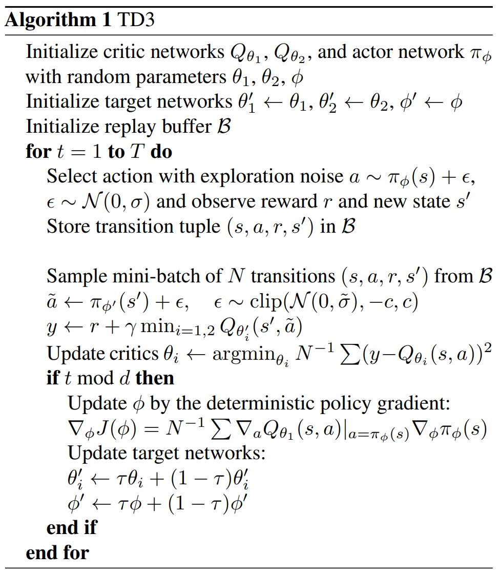
In general, the TD3 works in the following way. It maintains a pair of critics and a single actor. For each step (after every time interval in our simulation), we update both critics towards the minimum target value of actions selected by the current target policy:

\[\begin{split}& y=r+\gamma \min _{i=1,2} Q_{\theta_i^{\prime}}\left(s^{\prime}, \pi_{\phi^{\prime}}\left(s^{\prime}\right)+\epsilon\right), \\ & \epsilon \sim \operatorname{clip}(\mathcal{N}(0, \sigma),-c, c)\end{split}\]

Every \(d\) iterations, which is implemented with the train_freq, the policy is updated with respect to \(Q_{\theta_1}\) following the deterministic policy gradient algorithm (Silver et al., 2014). TD3 is summarized in the following picture from the authors of the original paper (Fujimoto, Hoof and Meger, 2018).

The steps in the algorithm are translated to implementations in ASSUME in the following way. The initialization of the actors and critics is done by the assume.reinforcement_learning.algorithms.matd3.TD3.initialize_policy() function, which is called in the learning role. The replay buffer needs to be stable across different episodes, which corresponds to runs of the entire simulation, hence it needs to be detached from the entities of the simulation that are killed after each episode, like the learning role. Therefore, it is initialized independently and given to the learning role at the beginning of each episode. For more information regarding the buffer see Replay Buffer.

The core of the algorithm is embodied by the assume.reinforcement_learning.algorithms.matd3.TD3.update_policy() in the learning algorithms. Here, the critic and the actor are updated according to the algorithm.

The network architecture for the actor in the RL algorithm can be customized by specifying the network architecture used. In Stable Baselines3 they are also referred to as “policies”. The architecture is defined as a list of names that represent the layers of the neural network. For example, to implement a multi-layer perceptron (MLP) architecture for the actor, you can set the “actor_architecture” config item to [“mlp”]. This will create a neural network with multiple fully connected layers.

Other available options for the “policy” include Long-Short-Term Memory (LSTMs). The architecture for the observation handling is implemented from [2]. Note, that the specific implementation of each network architecture is defined in the corresponding classes in the codebase. You can refer to the implementation of each architecture for more details on how they are implemented.

[2] Y. Ye, D. Qiu, J. Li and G. Strbac, “Multi-Period and Multi-Spatial Equilibrium Analysis in Imperfect Electricity Markets: A Novel Multi-Agent Deep Reinforcement Learning Approach,” in IEEE Access, vol. 7, pp. 130515-130529, 2019, doi: 10.1109/ACCESS.2019.2940005.

Replay Buffer

This chapter gives you an insight into the general usage of buffers in reinforcement learning and how they are implemented in ASSUME.

Why do we need buffers?

In reinforcement learning, a buffer, often referred to as a replay buffer, is a crucial component in algorithms like for Experience Replay. It serves as a memory for the agent’s past experiences, storing tuples of observations, actions, rewards, and subsequent observations.

Instead of immediately using each new experience for training, the experiences are stored in the buffer. During the training process, a batch of experiences is randomly sampled from the replay buffer. This random sampling breaks the temporal correlation in the data, contributing to a more stable learning process.

The replay buffer improves sample efficiency by allowing the agent to reuse and learn from past experiences multiple times. This reduces the reliance on new experiences and makes better use of the available data. It also helps mitigate the effects of non-stationarity in the environment, as the agent is exposed to a diverse set of experiences.

Overall, the replay buffer is instrumental in stabilizing the learning process in reinforcement learning algorithms, enhancing their robustness and performance by providing a diverse and non-correlated set of training samples.

How are they used in ASSUME?

In principal ASSUME allows for different buffers to be implemented. They just need to adhere to the structure presented in the base buffer. Here we will present the different buffers already implemented, which is only one, yet.

The simple replay buffer

The replay buffer is currently implemented as a simple circular buffer, where the oldest experiences are discarded when the buffer is full. This ensures that the agent is always learning from the most recent experiences. Yet, the buffer is quite large to store all observations also from multiple agents. It is initialised with zeros and then gradually filled. Basically after every step of the environment the data is collected in the learning role which sends it to the replay buffer by calling its add function.

After a certain round of training runs which is defined in the config file the RL strategy is updated by calling the update function of the respective algorithms which calls the sample function of the replay buffer. The sample function returns a batch of experiences which is then used to update the RL strategy. For more information on the learning capabilities of ASSUME, see Introduction to Reinforcement Learning.